how to draw 3d graph in maple

Matplotlib was introduced keeping in mind, simply two-dimensional plotting. Just at the time when the release of 1.0 occurred, the 3d utilities were developed upon the 2d and thus, we accept 3d implementation of data available today! The 3d plots are enabled by importing the mplot3d toolkit. In this commodity, nosotros will deal with the 3d plots using matplotlib.
Case:

Python3

import numpy as np

import matplotlib.pyplot every bit plt

fig = plt.figure()

ax = plt.axes(projection = '3d' )

Output:

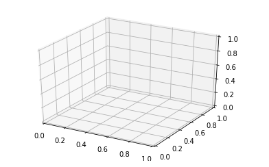
With the above syntax three -dimensional axes are enabled and data can be plotted in three dimensions. iii dimension graph gives a dynamic approach and makes information more interactive. Similar two-D graphs, we can utilize dissimilar ways to represent 3-D graph. We can make a scatter plot, contour plot, surface plot, etc. Let's have a expect at different 3-D plots.

Plotting iii-D Lines and Points

Graph with lines and point are the simplest 3 dimensional graph. ax.plot3d and ax.besprinkle are the function to plot line and point graph respectively.
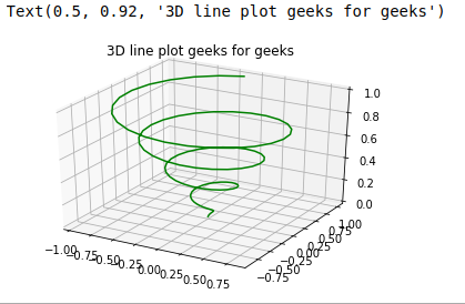
Case ane: 3 dimensional line graph

Python3

from mpl_toolkits import mplot3d

import numpy every bit np

import matplotlib.pyplot as plt

fig = plt.figure()

ax = plt.axes(project = '3d' )

z = np.linspace( 0 , ane , 100 )

x = z * np.sin( 25 * z)

y = z * np.cos( 25 * z)

ax.plot3D(10, y, z, 'green' )

ax.set_title( '3D line plot geeks for geeks' )

plt.bear witness()

Output:

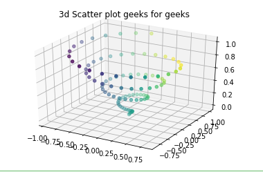
Case 2: iii dimensional scattered graph

Python3

from mpl_toolkits import mplot3d

import numpy every bit np

import matplotlib.pyplot as plt

fig = plt.figure()

ax = plt.axes(projection = '3d' )

z = np.linspace( 0 , ane , 100 )

x = z * np.sin( 25 * z)

y = z * np.cos( 25 * z)

c = x + y

ax.besprinkle(x, y, z, c = c)

ax.set_title( '3d Scatter plot geeks for geeks' )

plt.show()

Output:

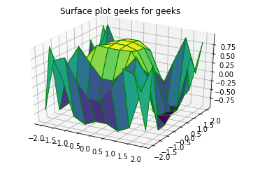
Plotting Surface graphs and Wireframes

Surface graph and Wireframes graph work on gridded data. They take grid value and plot it on 3-dimensional surface.
Example one: Surface graph

Python3

from mpl_toolkits import mplot3d

import numpy as np

import matplotlib.pyplot as plt

x = np.outer(np.linspace( - 2 , 2 , ten ), np.ones( 10 ))

y = x.re-create().T

z = np.cos(10 * * 2 + y * * 3 )

fig = plt.figure()

ax = plt.axes(projection = '3d' )

ax.plot_surface(x, y, z, cmap = 'viridis' , edgecolor = 'light-green' )

ax.set_title( 'Surface plot geeks for geeks' )

plt.show()

Output:

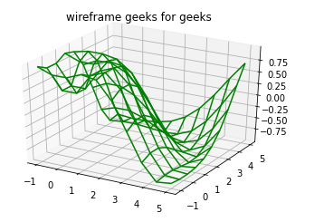
Example 2: Wireframes

Python3

from mpl_toolkits import mplot3d

import numpy as np

import matplotlib.pyplot as plt

def f(x, y):

return np.sin(np.sqrt(x * * 2 + y * * ii ))

x = np.linspace( - 1 , 5 , 10 )

y = np.linspace( - 1 , v , 10 )

X, Y = np.meshgrid(x, y)

Z = f(10, Y)

fig = plt.figure()

ax = plt.axes(projection = '3d' )

ax.plot_wireframe(Ten, Y, Z, color = 'green' )

ax.set_title( 'wireframe geeks for geeks' );

Output:

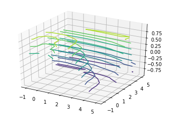
Plotting Contour Graphs

Profile graph takes all the input data in two-dimensional regular grids, and the Z data is evaluated at every point.Nosotros use ax.contour3D role to plot a contour graph.
Example:

Python3

from mpl_toolkits import mplot3d

import numpy as np

import matplotlib.pyplot as plt

def f(10, y):

return np.sin(np.sqrt(x * * 2 + y * * 3 ))

x = np.linspace( - 1 , v , x )

y = np.linspace( - i , v , 10 )

10, Y = np.meshgrid(ten, y)

Z = f(Ten, Y)

fig = plt.figure()

ax = plt.axes(projection = '3d' )

ax.contour3D(X, Y, Z)

Output:

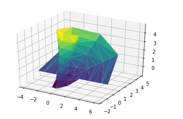
Plotting Surface Triangulations

The higher up graph is sometimes overly restricted and inconvenient. So by this method, we employ a prepare of random draws. The function ax.plot_trisurf is used to draw this graph. It is not that clear but more than flexible.
Example:

Python3

from mpl_toolkits import mplot3d

import numpy every bit np

import matplotlib.pyplot every bit plt

theta = 2 * np.pi * np.random.random( 100 )

r = 6 * np.random.random( 100 )

x = np.ravel(r * np.sin(theta))

y = np.ravel(r * np.cos(theta))

z = f(10, y)

ax = plt.axes(projection = '3d' )

ax.scatter(x, y, z, c = z, cmap = 'viridis' , linewidth = 0.25 );

ax = plt.axes(project = '3d' )

ax.plot_trisurf(x, y, z, cmap = 'viridis' , edgecolor = 'greenish' );

Output:

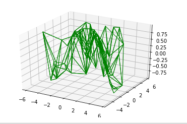
Plotting Möbius strip

Möbius strip also called the twisted cylinder, is a one-sided surface without boundaries. To create the Möbius strip think almost its parameterization, it's a ii-dimensional strip, and we need two intrinsic dimensions. Its bending range from 0 to 2 pie around the loop and width ranges from -one to 1.
Example:

Python3

from mpl_toolkits import mplot3d

import numpy as np

import matplotlib.pyplot as plt

from matplotlib.tri import Triangulation

theta = np.linspace( 0 , two * np.pi, 10 )

west = np.linspace( - ane , five , 8 )

w, theta = np.meshgrid(w, theta)

phi = 0.5 * theta

r = i + westward * np.cos(phi)

ten = np.ravel(r * np.cos(theta))

y = np.ravel(r * np.sin(theta))

z = np.ravel(w * np.sin(phi))

tri = Triangulation(np.ravel(west), np.ravel(theta))

ax = plt.axes(projection = '3d' )

ax.plot_trisurf(x, y, z, triangles = tri.triangles,

cmap = 'viridis' , linewidths = 0.two );

Output:

johnsonacom1978.blogspot.com

Source: https://www.geeksforgeeks.org/three-dimensional-plotting-in-python-using-matplotlib/

Share this post